Policy Search
- Policy Search
- Intro
- Difference between Policy Search and Value-based RL
- Policy Iteration
- Plain Policy Gradient
- Likelihood Ratio Gradient and REINFORCE
- G(PO)MDP
- Gauss-Newton
- Natural Policy Gradient
- Natural Actor-Critic
Intro
- Policy Search uses
- exploration
- evaluation
- updates
- based on experience data
- not model-based
-
not learning a value func first
- value based solution inefficient for large or high-dimensional spaces

Difference between Policy Search and Value-based RL
- PS is guaranteed to converge
- good for high dimensional spaces
- can learn from demonstration Disadvantage of PS: Computationally Inefficient (see video)
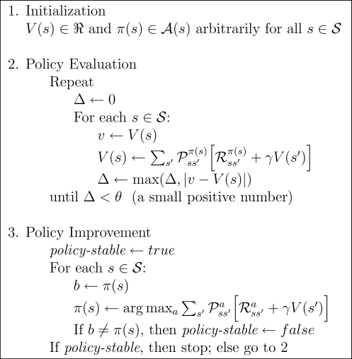
Policy Iteration
while (not converged)
  # Exploration:
  Generate Trajectories D using π(θ_k)
  # Evaluation:
  Check Quality of π(θ_k; D)
  # Update:
  Make π(θ_{k+1}) using evaluations and trajectories
or
Plain Policy Gradient
Update the policy via updating its parametrization
input: policy parametrization θh
for i=1 to  I do
    generate policy variation Δθi
    estimate J^i≈J(θh+Δθi) = ⟨∑Hk=0akrk⟩ from roll-out
    estimate J^ref , e.g., J^ref=J(θh−Δθi) from roll-out
    compute ΔJ^i≈J(θh+Δθi)−Jref
end for
return gradient estimate g_FD(θ) = (ΔΘ^T ΔΘ)^−1 ΔΘ^T ΔJ
gradient update: θ = θ + α g_FD(θ)
Works well if J i not to noisy
Likelihood Ratio Gradient and REINFORCE
This does not need parametrization. Baseline b is introduced to reduce variance. It vanishes for infinite data. Allows to use non-biased estimate gradients.

Advantages of this approach: Besides the theoretically faster convergence rate, likelihood ratio gradient methods have a variety of advantages in comparison to finite difference methods when applied to robotics. As the generation of policy parameter variations is no longer needed, the complicated control of these variables can no longer endanger the gradient estimation process. Furthermore, in practice, already a single roll-out can suffice for an unbiased gradient estimate viable for a good policy update step, thus reducing the amount of roll-outs needed. Finally, this approach has yielded the most real-world robotics results (Peters & Schaal, 2008) and the likelihood ratio gradient is guaranteed to achieve the fastest convergence of the error for a stochastic system. Disadvantages of this approach: When used with a deterministic policy, likelihood ratio gradients have to maintain a system model. Such a model can be very hard to obtain for continuous states and actions, hence, the simpler finite difference gradients are often superior in this scenario. Similarly, finite difference gradients can still be more useful than likelihood ratio gradients if the system is deterministic and very repetitive. Also, the practical implementation of a likelihood ratio gradient method is much more demanding than the one of a finite difference method.
G(PO)MDP
This aims to reduce the variance again by a baseline

Gauss-Newton
- second-order policy gradient
Natural Policy Gradient
Trying to use the actual gradient of the state instead of a scaled version.

Natural Actor-Critic
initialize θ0
For t = 0 : ∞ (until convergence)
  choose an action at from μθt (at |st )
  Take at , observe rt , and st+1 .
  Compute TD error: δt = rt + γφ(st+1 , at+1 )^T wt − φ(st , at )^T wt .
  Critic update: wt+1 = wt + αδt φ(st , at )
  Actor update: θt+1 = θt + βφ(st , at )φ(st , at )^T wt
end For